Théorie du Champ Electromagnétique (2025-2026)
Résumé de section
-
Electromagnetic field theory studies the interplay of electric and magnetic fields through Maxwell's equations, covering static fields, time-varying phenomena, and wave propagation essential for engineering applications.
Lessons typically span vector calculus basics, electrostatics/magnetostatics, and dynamic fields leading to EM waves, with practical examples in circuits and antennas.
Work focuses on solving boundary problems, computing potentials/fields, and analyzing transmission lines or radiation patterns to build analytical skills.
-
Chapter 1 introduces electrostatic field theory, focusing on fields from stationary charges in equilibrium.
Coulomb's law defines force between charges, leading to electric field E and Gauss's law ∫ E · dA = Q_enc/ε₀ for flux calculations. Electric potential V satisfies E = -∇V, with capacitors illustrating energy storage (½CV²).
Boundary value problems use Laplace's equation ∇²V = 0 for conductors and dielectrics, foundational for circuits and field mapping.
-
Chapter 2 delves into magnetostatic field theory, analyzing steady magnetic fields produced by constant currents, building on electrostatics principles.
It covers the Biot-Savart law for field computation from current elements, Ampère's circuital law ∮ H · dl = I_enc for symmetric cases, and magnetic vector potential A where B = ∇ × A. Materials introduce B, H, and M relations via permeability μ.
Topics include solenoids, toroids, force on current-carrying wires (F = I L × B), and torque on magnetic dipoles, essential for motors and transformers.
-
Chapter 3 introduces time-dependent regimes using the Quasi-Stationary Regime approximation (ARQS), valid for low-frequency variations where propagation effects are negligible.
ARQS assumes spatial uniformity over the observation domain at each instant, neglecting displacement current in Maxwell-Ampère's law relative to conduction current. This simplifies analysis of induction phenomena, like varying magnetic fields inducing emfs in circuits.
Focuses on time-varying fields from oscillating currents or dipoles, deriving retarded potentials while approximating static-like solutions for antennas and slow motions. Prepares for full wave propagation in later chapters.
-
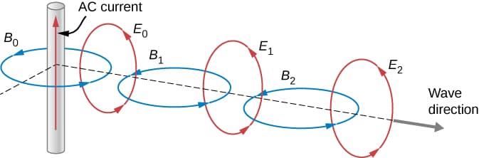
Chapter 4 explores time-varying Maxwell's equations, emphasizing their role in generating electromagnetic waves that propagate at a constant speed in free space.
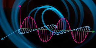
Starting from Faraday's and Ampere-Maxwell laws, the chapter derives the wave equation for E and H fields, revealing wave speed unifying electricity, magnetism, and light.Fields must be transverse (E ⊥ H ⊥ propagation direction), with mutual induction sustaining propagation, setting the stage for plane wave analysis.
-
hapter 5 covers the propagation of electromagnetic fields, focusing on plane waves in free space and lossless media derived from Maxwell's equations.
Time-harmonic fields satisfy the Helmholtz equation ∇²E + k²E = 0, where k = ω√(με) is the wavenumber. Uniform plane waves propagate as E = E₀ e^{-j k · r}, with speed c = 1/√(με).
Intrinsic impedance η = √(μ/ε) relates E and H fields; Poynting vector S = (1/2) Re(E × H*) gives time-average power flow. In dielectrics, waves attenuate negligibly if lossless, building to interface interactions in later chapters.
-
Chapter 6 examines reflection and transmission of electromagnetic plane waves at dielectric interfaces, using Maxwell's boundary conditions and Fresnel equations.
For normal incidence, reflection coefficient r = (η₂ - η₁)/(η₂ + η₁) determines reflected/transmitted amplitudes based on impedances η₁ and η₂. Oblique cases involve polarization (TE/TM), Snell's law, and Brewster's angle for zero reflection.